GEOG 337 LAB 3
Goals and Background
Lab three is intended for our class to understand and use the different ArcGIS tools that are needed to delineate watersheds. Recognizing and analyzing watersheds is extremely important in geography, specifically physical geography. Additionally, hydro-scientists and environmentalists alike can benefit from understanding the connectivity between different watersheds. They are significant when studying pollution effects and water flow data on a region or regions. An example of this would be recording the quality and amount of water that flows through a park or is entering a lake. Thus, it is useful for many to practice identifying and delineating watersheds in ArcGIS for land and water management.
This lab focuses on one watershed that has water flowing through Adirondack Park in New York."Adirondack Park is a protected area in northeastern New York that encompasses more than 6 million acres (24,700 square kilometers [km2]), which makes it the largest park in the contiguous United States. Although protected, much of the park is privately owned land, which is used mostly for forestry, agriculture, and recreation. Given its size and variety of uses, it is important to understand the sources and flow of water in the park," (Curtis). Using different tools of data collection and processing, the goal of this lab was to delineate different watershed sources of Adirondack park and analyze some information from each watershed.
Methods
Many different tools and methods were used to create our watershed maps. There were three general methods used: data collection, data processing, and watershed delineation. Each one used different tools within ArcGIS to create the final map. Collecting data first included downloading the specific shapefile for Adirondack Park and unzipping it to use with the hydrology data collected by Caitlin Curtis, our GIS professor. We also used a DEM (digital elevation model) from ArcGIS online. Processing the data involved overlaying the information before buffering the park boundary and making it easier to avoid watershed issues later on. Before overlaying each layer, we had to manipulate everything to make sure it was in the same projection and coordinate system. We also had to clip them all to the same boundaries.
After downloading and processing the data, we are ready to delineate the watersheds. Before creating this, we had to make many input datasets in order to have an output that fits what we wanted. The input datasets that had to be created were: flow direction, filled sinks, water accumulation, a source raster, and stream link. Flow direction was created using the spatial analysis tool under hydrology and flow direction. We then had to fill the sinks using the hydrology fill tool in order to raise their elevation to the cells surrounding them. Water accumulation and channel creations were determined by the spatial analyst tool under hydrology, called flow accumulation. Then, we created a source raster which was the input for our watershed delineation. To do this, we had to pick a threshold for the minimum number of cells that flow before it is designated as a stream cell. "This value ultimately determines the size and number of watersheds delineated and must be chosen carefully," (Curtis). Then we had to identify each stream reach by using the stream link tool under hydrology. Finally, we were able to create our watersheds using the watershed tool. This gave us our final maps to create and manipulate.
Results and Questions
1.Capture your final map output from Step 14, with all appropriate map elements.
After going through and finishing the lab "tutorial," it was time to practice some of the different ways we could manipulate the watershed data that we had created. This was done in the form of questions from Caitlin Curtis, our class professor. Each question started off with the base final map created from the tutorial. This base map is seen in Figure 1.0 and associated with the first question, asking to capture our final maps.
2.How many watersheds did your analysis yield?
My analysis yielded 96 watersheds, as found in the attribute table.

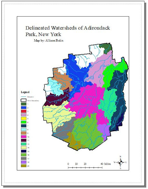
3.Change your DEM cell size to 120 m in step 15 (under Process Data) and then repeat the Delineate Watershed steps. How do the results vary in terms of number of watersheds? Why? Capture your output map.
As seen in Figure 1.1, I only had 20 watersheds. This is because I changed the digital elevation cell size to 120 instead of 60, making the cells much bigger. Because they’re bigger, they take up more space in the area, thus allowing for less watersheds to make up the region than before.
4.Change your source raster threshold to 100,000 and then 500,000. How many watersheds do you get in each case? Why do the results vary?
(still with DEM cell size at 120 but using feature classes from #1)
5.Compare your created vector streams file (from the first, 60m DEM) to the original hydro_utm83c file. How do they differ and why? Capture a map displaying both.
The vector streams differ from the normal streams because they are less detailed, vs the streams that are within the boundary are attached to the same coordinate system and can be more detailed with its links. The vector streams are attached to the flow direction and not necessarily the actual stream. The map captured showing this can be seen in Figure 1.2.
6.Open the vector streams attribute table. What are the from_node and to_node fields,and why are they important?
This determines the direction that the stream is taking. Streamflow does not always have a north to south direction, and the to and from nodes can show the directionality that each stream takes. This also helps with identification and analyzing of watersheds.

Sources
Caitlin Curtis. University of Wisconsin- Eau Claire
Adirondack Park boundary shapefile from the New York State GIS Clearinghouse at
http://gis.ny.gov/
Hydrology shapefile from Cornell University's Geospatial Information Repository (CUGIR) site at http://cugir.mannlib.cornell.edu/index.jsp
A 30-arc-second digital elevation model (DEM) of North America accessed from ArcGIS online.
Lab three is intended for our class to understand and use the different ArcGIS tools that are needed to delineate watersheds. Recognizing and analyzing watersheds is extremely important in geography, specifically physical geography. Additionally, hydro-scientists and environmentalists alike can benefit from understanding the connectivity between different watersheds. They are significant when studying pollution effects and water flow data on a region or regions. An example of this would be recording the quality and amount of water that flows through a park or is entering a lake. Thus, it is useful for many to practice identifying and delineating watersheds in ArcGIS for land and water management.
This lab focuses on one watershed that has water flowing through Adirondack Park in New York."Adirondack Park is a protected area in northeastern New York that encompasses more than 6 million acres (24,700 square kilometers [km2]), which makes it the largest park in the contiguous United States. Although protected, much of the park is privately owned land, which is used mostly for forestry, agriculture, and recreation. Given its size and variety of uses, it is important to understand the sources and flow of water in the park," (Curtis). Using different tools of data collection and processing, the goal of this lab was to delineate different watershed sources of Adirondack park and analyze some information from each watershed.
Methods
Many different tools and methods were used to create our watershed maps. There were three general methods used: data collection, data processing, and watershed delineation. Each one used different tools within ArcGIS to create the final map. Collecting data first included downloading the specific shapefile for Adirondack Park and unzipping it to use with the hydrology data collected by Caitlin Curtis, our GIS professor. We also used a DEM (digital elevation model) from ArcGIS online. Processing the data involved overlaying the information before buffering the park boundary and making it easier to avoid watershed issues later on. Before overlaying each layer, we had to manipulate everything to make sure it was in the same projection and coordinate system. We also had to clip them all to the same boundaries.
After downloading and processing the data, we are ready to delineate the watersheds. Before creating this, we had to make many input datasets in order to have an output that fits what we wanted. The input datasets that had to be created were: flow direction, filled sinks, water accumulation, a source raster, and stream link. Flow direction was created using the spatial analysis tool under hydrology and flow direction. We then had to fill the sinks using the hydrology fill tool in order to raise their elevation to the cells surrounding them. Water accumulation and channel creations were determined by the spatial analyst tool under hydrology, called flow accumulation. Then, we created a source raster which was the input for our watershed delineation. To do this, we had to pick a threshold for the minimum number of cells that flow before it is designated as a stream cell. "This value ultimately determines the size and number of watersheds delineated and must be chosen carefully," (Curtis). Then we had to identify each stream reach by using the stream link tool under hydrology. Finally, we were able to create our watersheds using the watershed tool. This gave us our final maps to create and manipulate.
Results and Questions
1.Capture your final map output from Step 14, with all appropriate map elements.
After going through and finishing the lab "tutorial," it was time to practice some of the different ways we could manipulate the watershed data that we had created. This was done in the form of questions from Caitlin Curtis, our class professor. Each question started off with the base final map created from the tutorial. This base map is seen in Figure 1.0 and associated with the first question, asking to capture our final maps.
2.How many watersheds did your analysis yield?
My analysis yielded 96 watersheds, as found in the attribute table.

Figure 1.0 Map result for question #1.
As seen in Figure 1.1, I only had 20 watersheds. This is because I changed the digital elevation cell size to 120 instead of 60, making the cells much bigger. Because they’re bigger, they take up more space in the area, thus allowing for less watersheds to make up the region than before.
4.Change your source raster threshold to 100,000 and then 500,000. How many watersheds do you get in each case? Why do the results vary?
(still with DEM cell size at 120 but using feature classes from #1)
Number of watersheds with source raster
threshold at 100,000: 35 watersheds
Source raster threshold at 500,000: 7
watersheds
The results are varied because less and less streams are meeting the raster threshold as it gets higher. When less streams meet the threshold, less watersheds can be delineated.

Figure 1.1 Map result for question #3.
The vector streams differ from the normal streams because they are less detailed, vs the streams that are within the boundary are attached to the same coordinate system and can be more detailed with its links. The vector streams are attached to the flow direction and not necessarily the actual stream. The map captured showing this can be seen in Figure 1.2.
6.Open the vector streams attribute table. What are the from_node and to_node fields,and why are they important?
This determines the direction that the stream is taking. Streamflow does not always have a north to south direction, and the to and from nodes can show the directionality that each stream takes. This also helps with identification and analyzing of watersheds.

Figure 1.2 Map result for #5.
Sources
Caitlin Curtis. University of Wisconsin- Eau Claire
Adirondack Park boundary shapefile from the New York State GIS Clearinghouse at
http://gis.ny.gov/
Hydrology shapefile from Cornell University's Geospatial Information Repository (CUGIR) site at http://cugir.mannlib.cornell.edu/index.jsp
A 30-arc-second digital elevation model (DEM) of North America accessed from ArcGIS online.

Comments
Post a Comment